Machine Learning Notes

Tianyao (Till) Chen

May 1, 2020 4565 words 22 minutes

Contents

Introduction
- Types of Learning
Notations and Definitions
- Statistical Decision Theory
Fundamental Algorithms
Anatomy of a Learning Algorithm
Basic Practice
Neural Networks and Deep Learning
- Neural Networks
  - Multilayer Perceptron (Vanilla Neural Network)
  - Feed-Forward Neural Network Architecture
- Deep Learning
  - Convolutional Neural Network
  - Recurrent Neural Network
Problems and Solutions
Unsupervised Learning
References

Introduction

This post is about some basic machine learning concepts.

Types of Learning

Supervised learning

In a feature vector $x_i$ (i=1…N), a single feature is denoted by $x^j$ (j=1…D). And $y_i$ is the label.
The goal is to produce a model that takes a feature vector x as input and outputs the label.

Unsupervised learning

The goal is either to transform the input feature vector into another vector (dimensionality reduction) or into a value (clustering, outlier detection).

Semi-supervised learning

The dataset has both labeled and unlabeled (much higher quantity) data.
The same goal as supervised learning.
The hope is that the unlabeled data can help produce a better model. This is because a larger sample reflects better the probability distribution of the source of the labeled data.

Reinforcement learning

It perceives the state of the environment as a feature vector and then execute actions in every state, which bring rewards and move the machine to another state.
The goal is to learn a policy: a function that takes the feature vector as input and outputs an optimal action that maximizes the expected average reward.
It’s suited for problems whose decision making is sequential and the goal is long-term.

Notations and Definitions

$x_{l,u}^{(j)}$ in a neural net means the feature j of unit u in layer l.
$x$ is by default a column vector and $x^T$ a row vector. When vector is on the left side of a matrix, we usually do $x^TA$.
$argmax_{a \in A}f(a)$ returns the element a of the set A that maximizes f(a).
$\mathbb{E}[\hat\theta(S_X) = \theta]$, where $\hat\theta(S_X)$ is the unbiased estimator of some statistic $\theta$ (e.g. $\mu$) calculated using a sample $S_X$.
A hyperparameter is a parameter whose value is set before the learning process begins. By contrast, the values of other parameters are derived via training.
Model-based learning vs instance-based learning:
- Model-based: creates a model with parameters learned from the data. (Most supervised learning algorithms)
- Instance-based: uses the whole dataset as the model. Instead of performing explicit generalization, it compares new problem instances with instances seen in training (e.g. kNN).
Shallow vs deep learning:
- Shallow learning: learns the parameters of the model directly from the features of the training examples.
- Deep (neural network) learning: uses neural nets with more than one layer and learns the parameters from the outputs of the preceding layers instead.

Statistical Decision Theory

Quantitative outputs are called $Y$ with $Y = (Y_1,…,Y_K)^T$; and qualitative outputs are called $G$ with $G = (G_1,…,G_K)^T$ (group).
Loss functions:

$$L_2(y, y’) = (y-y’)^2$$

$$L_{0-1}(g, g’) = 0 \ (g=g’) \ or \ 1 \ (g\neq g’)$$

$$L_1(y,y’) = |y-y’|$$
Expected prediction error (EPE):

$$EPE(f)=E(L_2(Y,f(X)))$$

$$EPE(f)=E(L_{0-1}(G,f(X)))$$
The function f that minimizes EPE is give by: ($E(Y|X=x)$ is called a regressor/regression function)

$$f(x)=E(Y|X=x)$$
Bayes classifier:

$$f(x)=argmin_{g \in R_G}[1-p(g|x)] \Rightarrow$$

$$f(x)=\mathbf{g} \ if \ p(\mathbf{g}|x) = \max_{g \in R_G}p(g|x)$$
Expected squared prediction error of $\hat f$ at location $x_0$:

$$EPE(\hat f, x_0)=E(L_2(Y,f(X))|X=x_0)$$
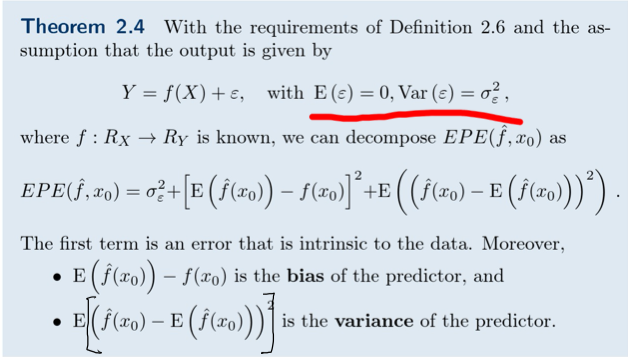
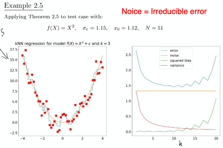
Error = Irreducible Error + $\text{Bias}^2$ + Variance

Fundamental Algorithms

Linear Regression

We want a model as a linear combination of features of example x ($w$ is a D-dimensional vector of parameters and b is a real number.):

$$f_{w,b}(x) = wx+b$$
We find the optimal values $w^{*}$ and $b^{*}$ by minimizing the cost function below (the empirical risk - the average loss):

$$\frac{1}{N}\sum_{i=1…N}(f_{w,b}(x_i)-y_i)^2$$
Overfitting: a model that predicts well for the training data but not for data unseen during training. Linear regression rarely overfits.
The squared loss is used since it’s convinent. The absolute loss function doesn’t have a continuous derivative, which makes it not smooth. Unsmooth functions create difficulties for optimization problems in linear algebra.
To find the extrema (minima or maxima), we can simply set the gradient to zero.
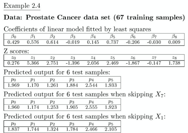
The linear model is an approximation for the regressor $E(Y|X)$ of the form: ($\beta_0$ is the intercept or bias)

$$f_{\beta}(X) = \beta_0+\sum_{j=1}^DX_j\beta_j$$
By using $\beta = (\beta_0,…,\beta_D)^T$ and $Z=(1,X_1,…,X_D)^T$, we can rewrite the model to:

$$f_{\beta}(Z)=Z^T\beta$$
The least squares estimator (parameter estimator $\gamma$):

$$\gamma = argmin_{\gamma}\sum_{i=1}^N(y_i-f_{\gamma}(x_i))^2$$
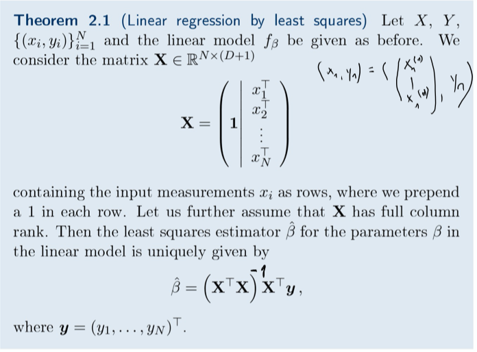
Solution for the estimator:
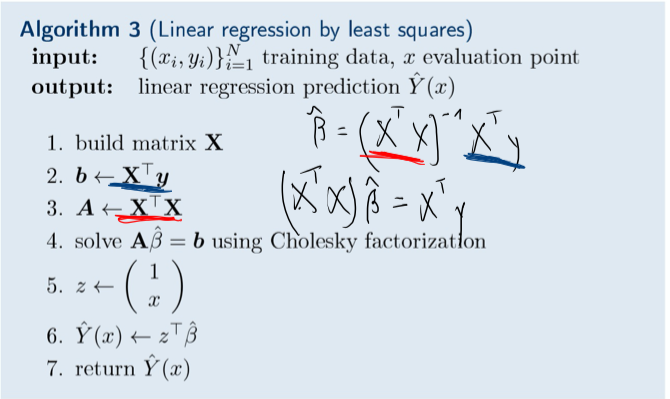
The algorithm:
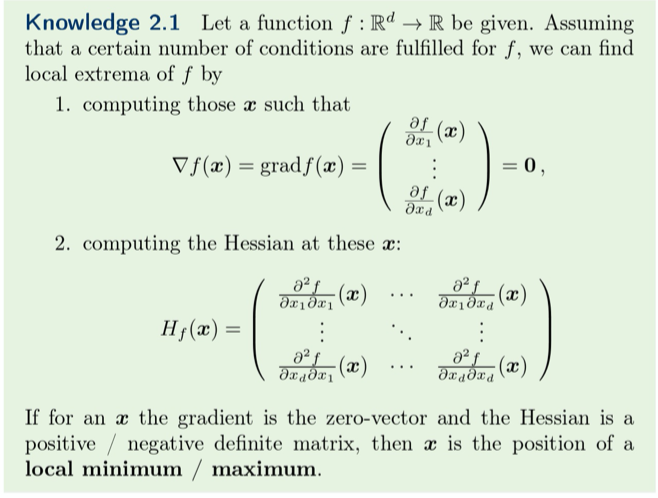
Find local minimum/maximum:

$$M \ \text{positive definite} \Leftrightarrow x^TMx>0 \ \text{for all }x \in \mathbb{R}^n \backslash \mathbf{0}$$

$$M \ \text{negative definite} \Leftrightarrow x^TMx<0 \ \text{for all }x \in \mathbb{R}^n \backslash \mathbf{0}$$
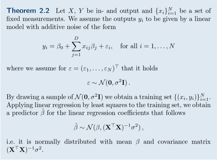
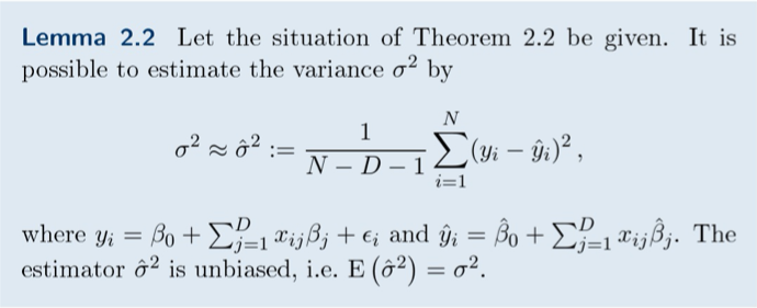
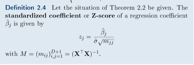
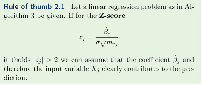
Statistical analysis with the additive noise:
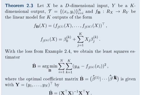
For a K-dimensional output:

Logistic Regression

Logistic regression is not a regression, but a classification learning algorithm. The names is because the mathematical formulation is similar to linear regression.
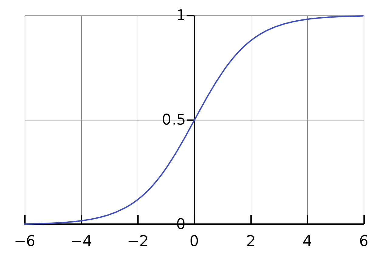
The standard logistic function or the sigmoid function:

$$f(x)=\frac{1}{1+e^{-x}}$$
The logistic regression model:

$$f(x)=\frac{1}{1+e^{-(wx+b)}}$$
For binary classification, we can say the label is positive if the probability is higher than or equal to 0.5.
We optimize by using the maximum likelihood (the goodness of fit) ($y_i$ is either 0 or 1):

$$L_{w,b}=\prod_{i=1…N}f_{w,b}(x_i)^{y_i}(1-f_{w,b}(x_i))^{1-y_i}$$
In practice, it’s more convenient to maximize the log-likelihood (since ln is a strictly increasing function, maximizing this is the same as maximizing its argument):

$$LogL_{w,b}=ln(L_{w,b})=\sum_{i=1}^Ny_iln(f_{w,b}(x_i)) + (1-y_i)ln(1-f_{w,b}(x_i))$$
Unlike linear regression, there’s no closed form solution. A typical numerical optimization procedure is gradient descent.

Decision Tree Learning

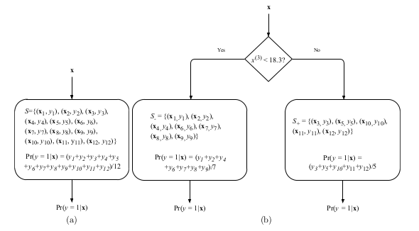
If the value is below a specific threshold, the left branch is followed. Otherwise, the right branch is followed. The decision is made about the class when the leaf node is reached.
We consider ID3 (Iterative Dichotomiser 3), which also optimizes the average log-likelihood like logistic regression. It does some approximately by constructing a nonparametric model $f_{ID3} = Pr(y=1|\mathbf{x})$.
Entropy is a measure of uncertainty about a random variable. We find a split that minimizes the entropy.

Support Vector Machine

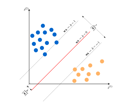
The model $f(\mathbf{x}) = sign(\mathbf{w^{*}x} - b^{*})$ (sign returns +1 if it’s positive and -1 if it’s negative) (The sign * means the optimal value.)
We prefer the hyperplane with the largest margin, which is the distance between the closest examples of two classes. A large margin contributes to a better generalization. We achieve this by minimizing the norm of $\mathbf{w}$: $||\mathbf{w}||$.

Dealing With Noise

We can use the hinge loss function: $\max (0, 1 - y_i(\mathbf{wx}_i - b))$ for data that’s not linearly separable.

Dealing with Inherent Non-Linearity (Kernels)

The kernel trick: use a function to implicitly transform the original space into a higher dimensional space during the cost function optimization. (We hope that data will be linearly separable in the transformed space).
We use kernel functions or simply kernels to efficiently work in higher-dimensional spaces without doing this transformation explicitly.
By using the kernel trick, we get rid of a costly transformation to the higher dimension and avoid computing their dot-product.
We can use the quadratic kernel $k(x_i, x_k) = (x_ix_k)^2$ here. Another widely used kernel is the RBF (radial basis function) kernel: $k(x, x^{’}) = exp(-\frac{||x-x^{’}||^2}{2\sigma^2})$. It has infinite dimensions. We can vary the hyperparameter $\sigma$ and choose wether to get a smooth of curvy decision boundary.

k-Nearest Neighbors (kNN)

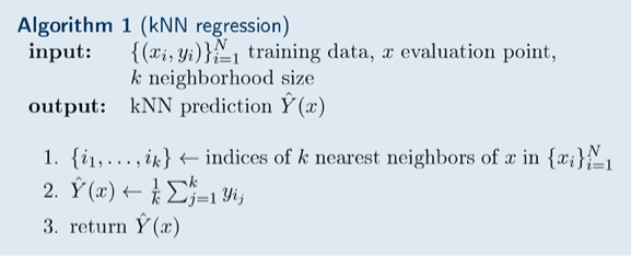
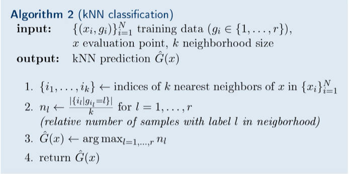
kNN is a non-parametric learning algorithm. Contrary to other learning algorithms that allow discarding the training data after the model is built, kNN keeps all training examples in memory.
The closeness of two examples is given by a distance function. Other than the Euclidean distance, we could also use the cosine similarity function ($0^{\circ}: 1; 90^{\circ}: 0; 180^{\circ}: -1$).
Algorithms
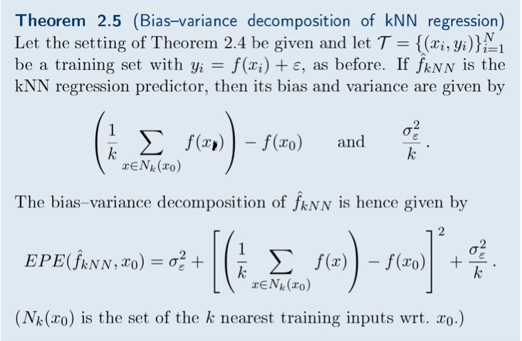
The bias-variance decomposition:
The bias-variance trade-off:
- k=1: if $x_0$ is in the training data, the bias = 0; the largest variance. (similar to overfitting)
- k=N: the largest bias (the predictor is constant); the smallest variance. (similar to underfitting)

Anatomy of a Learning Algorithm

Building blocks

A loss function
An optimization criterion based on the loss function (e.g. a cost function)
An optimization routine leveraging training data to find a solution to the optimization criterion.

Gradient Descent

To find a local minimum, start at some random point and takes step proportional (learning rate) to the negative of the gradient.
The gradient is calculated by taking the partial derivative for every parameter in the loss function: (take linear regression as an example)

$$l = \frac{1}{N}\sum_{i=1}^{N}(y_i-(wx_i+b))^2$$

$$\frac{\partial l}{\partial w} = \frac{1}{N}\sum_{i=1}^{N}-2x_i(y_i-(wx_i+b))$$

$$\frac{\partial l}{\partial b} = \frac{1}{N}\sum_{i=1}^{N}-2(y_i-(wx_i+b))$$
An epoch consists of using the training set entirely to update each parameter. (One sweep through full training data.) At each epoch, we update $w$ and $b$ ($\alpha$ is the learning rate):

$$w \leftarrow w - \alpha\frac{\partial l}{\partial w}$$

$$b \leftarrow b - \alpha\frac{\partial l}{\partial b}$$
Minibatch stochastic gradient descent is a version that speed up the computation by approximating the gradient using smaller batches.
Issues with batch GD:
- Might get stuck in local minimum.
- One update, very expensive for large N.
Stochastic gradient descent: use only one training sample to do update. (In each step, pick randomly and update)
- Each step is cheap.
- Can easily escape local minima.
- Many more steps necessary.
- Jumping around the solution.

Particularities

Some algorithms, like decision tree learning, can accept categorical features while others expect numerical values. All algorithms in scikit-learn expect numerical features.
Some algorithms, like SVM, allow weightings for each class. If the weighting is higher, the algorithm tries not to make errors in predicting training examples of this class.
Some classification models, like SVM and kNN, only output the class. Others, like logistic regression or decision trees, can also return the score between 0 and 1 (can be used as a confidence score).
Some classification algorithms - like decision trees, logistic regression, or SVM - build the model using the whole dataset at once. Others can be trained iteratively, one batch at a time.
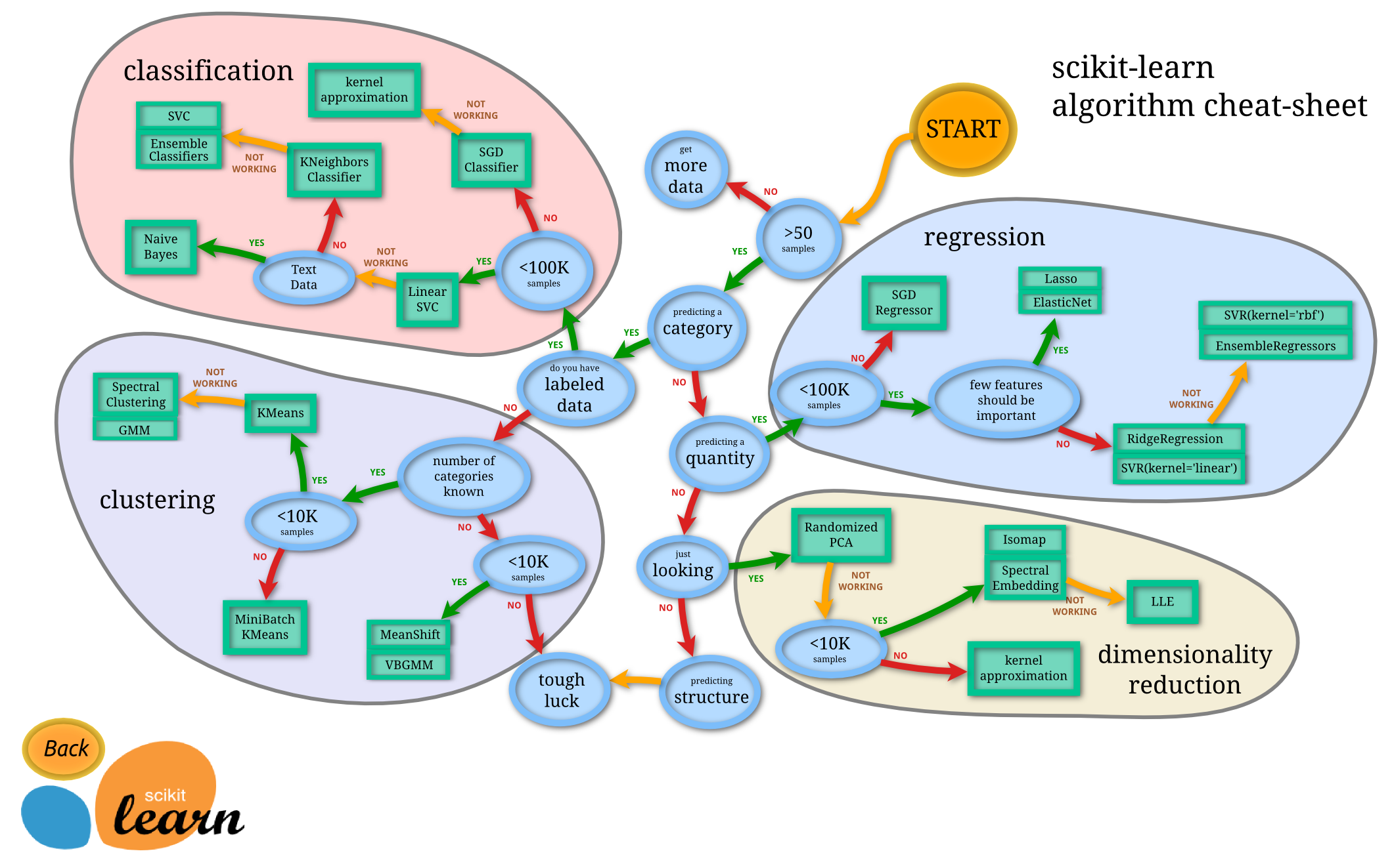
Some algorithms, like decision trees/SVM/kNN, can be used for both classification and regression, while others can only solve one type of problem.

Basic Practice

Feature Engineering

Feature engineering: the problem of transforming raw data into a dataset.
The role of the data analyst is to create informative features with high predictive power.
We say a model has a low bias when it predicts the training data well.

One-Hot Encoding (Categorical -> Numerical)

One-hot is a group of bits among which the legal combinations of values are only those with a single high (1) bit and all the others low (0). It transforms a categorical feature into several binary ones.
Example: red = [1,0,0]; yellow = [0,1,0]; green = [0,0,1].
When the ordering matters, we can just do: {poor, decent, good, excellent} -> {1, 2, 3, 4}.

Binning (Bucketing) (Numerical -> Categorical)

Binning converts a continuous feature in to multiple binary features called bins, typically based on value range.

Normalization

Normalization converts a numerical value into a value typically in the interval [-1,1] or [0,1], which increases the speed of learning:

$$\bar x^{(j)} = \frac{x^{(j)}-min^{(j)}}{max^{(j)}-min^{(j)}}$$

Standardization (Z-score Normalization)

Standardization rescales the feature values so that they have the properties of a standard normal distribution with $\mu = 0$ and $\sigma = 1$.
Standard scores or z-scores can be calculated as follows:

$$\hat x^{(j)} = \frac{x^{(j)} - \mu^{(j)}}{\sigma^{(j)}}$$
Normalization vs Standardization:
- Unsupervised learning - standardization.
- The distribution is close to a normal distribution - standardization.
- Have outliers - standardization (normalization will squeeze the normal values into a very small range).
- Other cases - normalization.

Dealing with Missing Features

Remove the examples with missing features
Use a learning algorithm that can deal with missing feature values.
Use Data imputation (the process of replacing missing data with substituted values)
- Replace the missing value with an average value.
- Replace the missing value with a value outside the normal range.
- Replace the missing value with a value in the middle of the range.
- Use the missing value as the target for a regression problem.
- Increase the dimensionality by adding a binary indicator feature.

Learning Algorithm Selection

Explainability
In-memory vs. out-of-memory (batch or incremental/online)
Number of features and examples (neural networks for a huge number of features)
Categorical vs. numerical features
Nonlinearity of the data (SVM/linear regression/linear kernel/logistic regression of lineraly separable data)
Training speed (neural networks are slow to train)
Prediction speed

Three Sets

Three sets:
- Training set (95%)
- Validation set (2.5%): choose the learning algorithm and find the best values of hyperparameters.
- Test set (2.5%): assess the model before delivery and production.
The last two are also called holdout sets, which are not used to build the model.

Underfitting and Overfitting

Underfitting: the model makes many mistakes on the training data - high bias.
- The model is too simple.
- The features are not informative enough.
Overfitting: the model predicts very well the training data but poorly the data from the holdout sets. - high variance (the error due to the sensitivity to small fluctuations in the training set) (variance is the difference in fits between data sets - consistency) (large generalization error)
- The model is too complex.
- Too many features but a small number of training examples.
The overfitting model learns the idiosyncrasies of the training set:
- the noise
- the sampling imperfection due to the small dataset size
- other artifacts extrinsic to the decision problem
Solutions for overfitting:
- Try a simply model
- Reduce the dimensionality
- Add more training data
- Regularization - the most widely used approach

Regularization

Regularization forces the learning algorithm to build a less complex model, which leads to a slightly higher bias but a much lower variance - the bias-variance tradeoff.
The two most widely used are L1 and L2 regularization, which add a penalizing term whose value is higher when the model is more complex.
For linear regression, L1 looks like this ($|\mathbf{w}| = \sum_{i=1}^D|w^{(j)}|$ and C is a hyperparameter), which tries to set most $w^{(j)}$ to value small values or zero (|| means abs here):

$$\min_{\mathbf{w},b} \left[C|\mathbf{w}| + \frac{1}{N}\sum_{i=1…N}(f_{\mathbf{w},b}(\mathbf{x}_i)-y_i)^2\right]$$
For linear regression, L2 looks like this (($||\mathbf{w}||^2 = \sum_{i=1}^D(w^{(j)})^2$):

$$\min_{\mathbf{w},b} \left[C||\mathbf{w}||^2 + \frac{1}{N}\sum_{i=1…N}(f_{\mathbf{w},b}(\mathbf{x}_i)-y_i)^2\right]$$
L1 produces a sparse model with most parameters equal to zero if C is large enough, which makes feature selection that decides which features are essential and increases explainability. L2 gives better results if our only goal is to maximize the performance on holdout sets. Plus L2 is differentiable - graident descent.
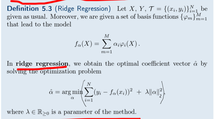
L1 and L2 are the special cases for elastic net regularization. L1 - lasso; L2 - ridge regularization.

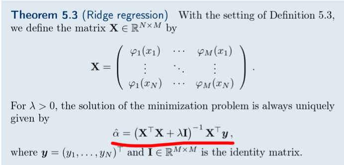
Shrinkage: Ridge Regression

Motivation: linear and basis expansion regression can lead to “non-full” column rank.
So we limit the size of coefficients (shrinkage) (a larger $\lambda$ means stronger shrinkage. The value is optimized by cross validation.):

Model Performance Assessment

For regression, we first compare our model with the mean model, which always predicts the average of the labels in the training data. If the fit or our model is better than the mean model, we compare the MSE (mean squared error) for the training and test data. If the MSE for the test data is substantially higher, it is a sign of overfitting.
For classification, we have the following metrics and tools:

Confusion Matrix

The confusion matrix is a table that summarizes how successful the classification model at predicting examples belonging to various classes.
Take a binary classification problem as an example:

spam (predicted) not_spam (predicted)

spam (actual) 23 (TP) 1 (FN)

not_spam (actual) 12 (FP) 556 (TN)

TP - True Positive; FN - False Negative;

FP - False Positive; TN - True Negative;

	spam (predicted)	not_spam (predicted)
spam (actual)	23 (TP)	1 (FN)
not_spam (actual)	12 (FP)	556 (TN)

Precision/Recall

Precision = $\frac{TP}{TP+FP}$ (TP/Positive Predictions)
Recall = $\frac{TP}{TP+FN}$ (TP/Positive Examples)

Accuracy

Accuracy = $\frac{TP+TN}{TP+TN+FP+FN}$

Cost-Sensitive Accuracy

When the classes have different importance, assign cost for FP and FN then multiply before calculating the accuracy.

Area under the ROC Curve (AUC)

ROC (Receiver Operating Characteristic) curve uses TPR (True Positive Rate – recall) and FPR (False Positive Rate – FP/FP+TN).
The higher the area under the ROC curve (AUC), the better the classifier.

Hyperparameter Tuning

Grid search: use continuous parameters in the logarithmic scale to generate all the combinations.
Some other techniques are Random Search (provide statistical distribution) and Bayesian (based on past evaluations).

Training Error

Definition ($\tau$ is the training set):

$$TE(\hat f, \tau) = \frac{1}{N}\sum_{i=1}^NL(y_i,\hat f(x_i))$$

Generalization/Test Error

Definition ($\tau$ is a sample of the random variable T):

$$ \begin{aligned} GE(\hat f, \tau) &= E_{X,Y}(L(Y, \hat f_T(X))|T=\tau) \\ &= \int_{R_Y}\int_{R_X}L(y, \hat f_T(x))\rho(x,y|\tau)dxdy \\ &= \int_{R_Y}\int_{R_X}L(y, \hat f_T(x))\frac{\rho(x,y,\tau)}{\rho_\tau\tau}dxdy \end{aligned} $$
Expected generalization/test error

$$ \begin{aligned} EGE(\hat f, \tau) &= E_T(E_{X,Y}(L(Y, \hat f_T(X))|T=\tau)) \\ &= \int_{R_T}(\int_{R_Y}\int_{R_X}L(y, \hat f_T(x))\rho(x,y|\tau)dxdy)\rho(\tau)d\tau \\ &= \int_{R_T}\int_{R_Y}\int_{R_X}L(y, \hat f_T(x))\rho(x,y,\tau) dxdyd\tau \end{aligned} $$

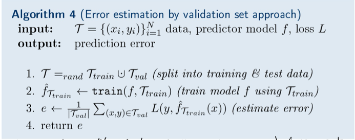
Validation Set Error Estimation

Cross-Validation

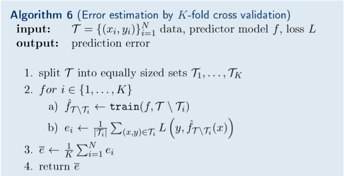
When we have few training examples, it could be prohibitive to have both validation and test set. So we can split the data into a training and a test set and use cross-validation on the training set to simulate a validation set.
Each subset of the training set is called a fold. Typically, a five-fold cross-validation is used in practice. We would train five models (use $F_2 F_3 F_4 F_5$ for model 1 and so on) and compute the value of the metric of interest on each validation set, from $F_1$ to $F_5$ and get the average score.
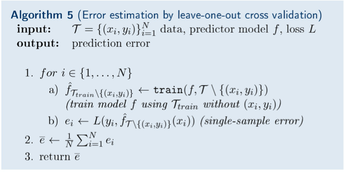
Leave-one-out cross validation:

Neural Networks and Deep Learning

Neural Networks

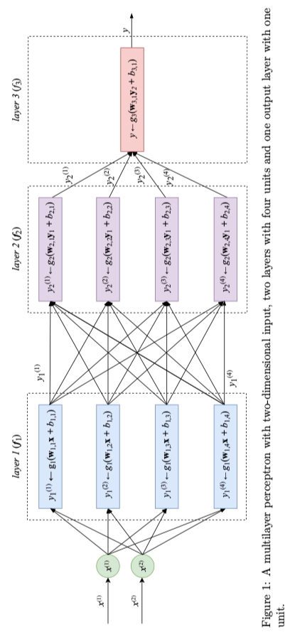
The function $f_{NN}$ is a nested function. So for a 3-layer neural network that returns a scalar:

$$y=f_{NN}(\mathbf{x}) = f_3(\mathbf{f}_2(\mathbf{f}_1(\mathbf{x})))$$

$\mathbf{f}_1$ and $\mathbf{f}_2$ are vector functions of the following form ($\mathbf{g}_l$ is the activation function - a fixed and chosen nonlinear function; $\mathbf{W}_l$ (a matrix) and $\mathbf{b}_l$ (a vector) are learned using gradient descent):

$$\mathbf{f}_l(\mathbf{z}) = \mathbf{g}_l(\mathbf{W}_l\mathbf{z} + \mathbf{b}_l)$$

Multilayer Perceptron (Vanilla Neural Network)

A multiplayer perceptron (MLP) is a class of a feed-forward neural network (FFNN). It has a fully-connected architecture.
In each rectangle unit:
1. All inputs of the unit are joined together to form an input vector.
2. The unit applies a linear transformation.
3. The unit applies an activation function.
An example (each unit’s parameters $w_{l,u}$ and $b_{l,u}$):
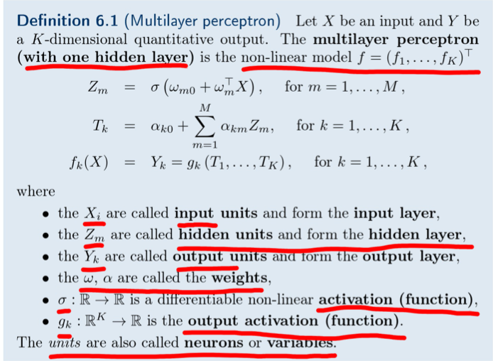
A more rigorous definition:
We can do regression/classification by optimizing the weight $\omega \ \alpha$.
- Highly non-linear, non-convex -> many local minima.
- $\omega \ \alpha$ often strongly underdetermined.
- No closed form formula -> use gradient descent.

Feed-Forward Neural Network Architecture

If we want to solve a regression or a classification problem, the last layer usually contains only one unit. If $g_{last}$ is linear, then the neural net is a regression model. If $g_{last}$ is a logistic function, it’s a binary classification model.
Any differentiable function can be chosen as $g_{l,u}$. And primary reason of such a nonlinear component is to allow the neural net to approximate nonlinear functions.
Popular choices for $g$ are the logistic function, TanH, and ReLU (rectified linear unit function):

$$tanh(z) = \frac{e^z - e^{-z}}{e^z + e^{-z}}$$

$$relu(z) = 0 \ \ if \ z < 0$$

$$relu(z)= z \ \ otherwise$$

Deep Learning

Deep learning refers to training neural networks with more than two non-ouput layers.
The two biggest challenges:
- Exploding gradient - use gradient clipping or $L_1$ $L_2$ regularization
- Vanishing gradient - use ReLU, LSTM, and skip connections (in residual neural networks)
Backpropagation is an efficient algorithm for computing gradients on neural networks using the chain rule. (It’s used to update the parameters.)
For overfitting:
- Early stopping in training.
- $L_2$ regularization.
- Add dropout layer.

Convolutional Neural Network

When our training examples are images, the input is very high-dimensional (each picture is a feature). If we use MLP, the optimization problem is likely to become intractable.
A convolutional neural network (CNN) is a special kind of FFNN that significantly reduces the number of parameters. Convolutional networks are simply neural networks that use convolution in place of general matrix multiplication in at least one of their layers.
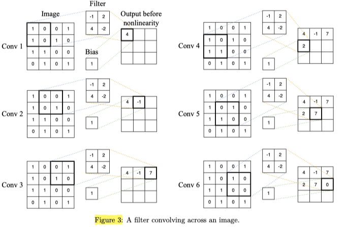
We use the moving window approach and then train multiple smaller regression models at once, each small regression model receiving a square patch as input. The goal of each small regression model is to detect a specific kind of pattern in the input patch. To detect some pattern, a small regression model has to learn the parameters of a matrix $\mathbf{F}$ (filter).
For example, if we have the following matrix $\mathbf{P}$ (patch) and $\mathbf{F}$, we can calculate the convolution of them. And the value is higher the more similar $\mathbf{F}$ is to $\mathbf{P}$. (The patch represents a pattern that looks like a cross.)
For convenience, there’s also a bias parameter b associated with each filter which is added to the result to a convolution.
One layer of a CNN consists of multiple convolution filters. Each filter of the first layer slides - or convolves - across the input image, left to right, top to bottom.
The filters and bias values are trainable parameters and are optimized using gradient descent with backpropagation.
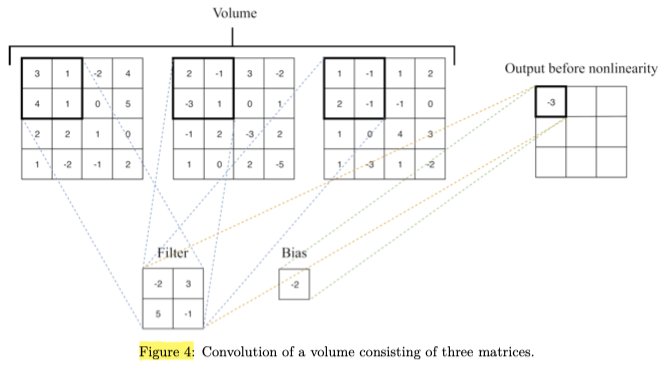
The subsequent layer treats the output of the preceding layer as a collection of image matrices. Such a collection is called a volume.
Stride is the step size of the moving window. We can also use paddings.
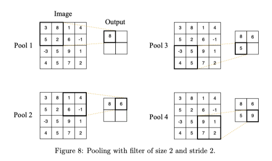
Pooling is a layer that applies a fixed operator, usually either max or average instead of applying a trainable filter. It increases the accuracy and improves the training speed by reducing the number of parameters. (The one below uses max.)

Recurrent Neural Network

RNN is the neural network whose connections between nodes form a directed graph along a temporal sequence. This allows it to exhibit temporal dynamic behavior.

Problems and Solutions

Basis Expansions

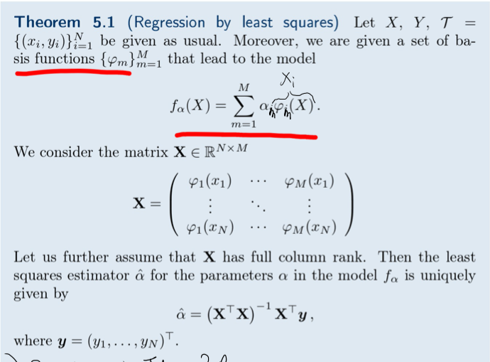
Basis expansion extends the linear model to a non-linear model. We achieve this by introducing basis functions $\phi_m (X)$.
Definition:
For quadratic polynomial regression, our basis functions will be: $\phi_1(x)=1, \ \phi_2(x)=x, \ \phi_3(x)=x^2$

Regression with Gaussian Kernel

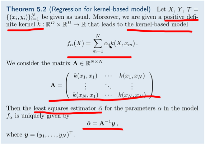
The Gaussian kernel ($\sigma^2$ is a scaler parameter, i.e. the variance or kernel width):

$$k(x,x’)=e^{-\frac{||x-x’||^2}{\sigma^2}}$$
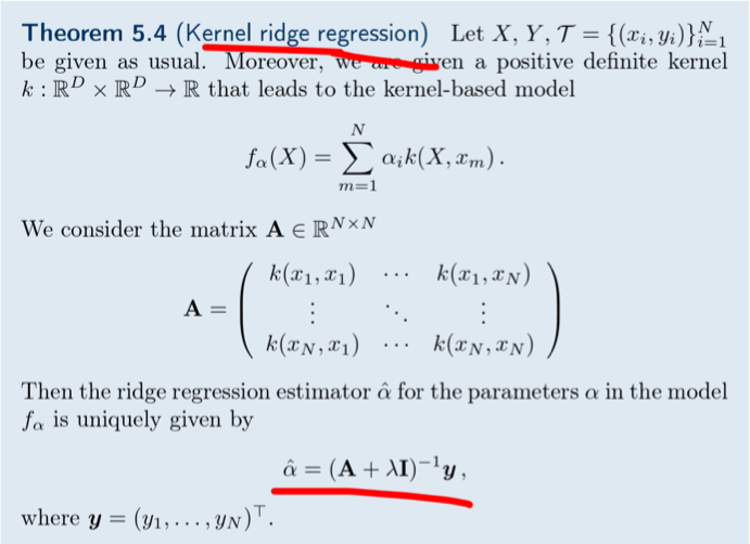
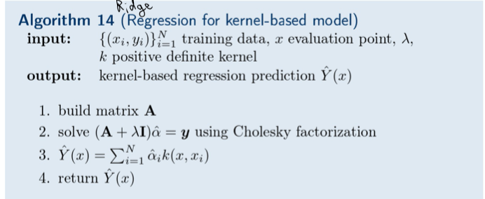
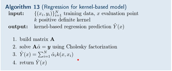
Regression for kernel-based model:

Kernel Regression

Kernel regression is a non-parametric method, which means there are no parameters to learn. The model is based on the data itself (like in kNN).
The simplest kernel regression looks like this (the function $k(\cdot)$ is called a kernel, which plays the role of a similarity function - $w_i$ is higher when x is similar to $x_i$):

$$f(x)=\frac{1}{N}\sum_{i=1}^{N}w_iy_i, \ where \ w_i = \frac{Nk(\frac{x_i - x}{b})}{\sum_{l=1}^Nk(\frac{x_l - x}{b})}$$
Kernels can have different forms, the most frequently used is the Gaussian kernel:

$$k(z)=\frac{1}{\sqrt{2\pi}}exp(\frac{-z^2}{2})$$

Classification

Decision boundary: the set of points at which the probability of x to be in either of the classes is equal:

$$\{x \in \mathbb{R}_X|p(1|x)=p(2|x)\}$$
The classification is linear if the decision boundaries are linear.
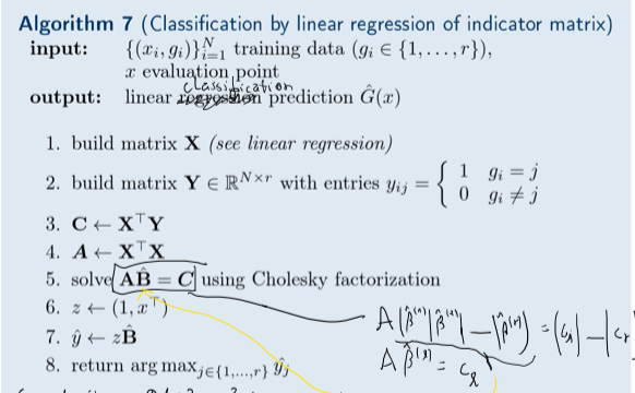
Classification by linear regression of indicator matrix:

Linear Discriminant Analysis

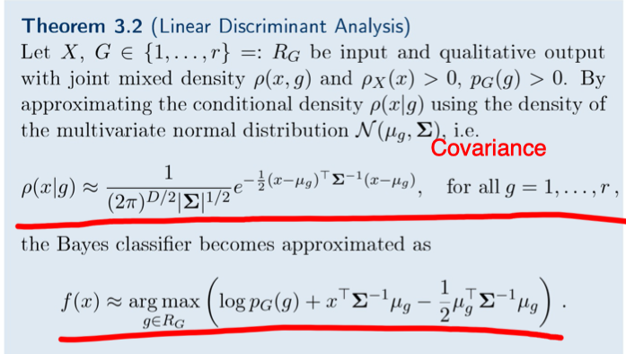
Linear Discriminant analysis (LDA) is a method used to find a linear combination of features that characterizes or separates two or more classes of objects or events. The resulting combination may be used as a linear classifier, or, more commonly, for dimensionality reduction before later classification.
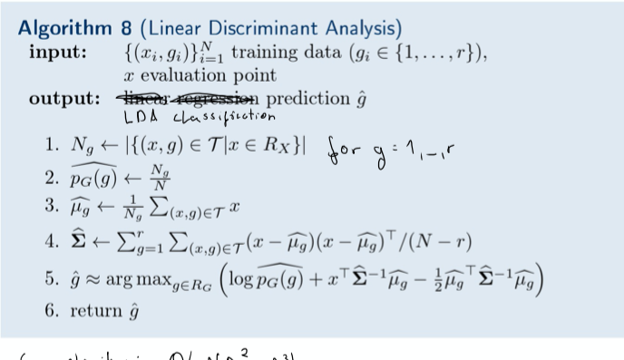
The mathematical definition and the algorithm:
LDA ia linear predictor.
A non-linear classification predictor can be obtained if we use $N(\mu_g, \Sigma_g)$ instead of $N(\mu_g, \Sigma)$, i.e. a class dependent covariance.

Ensemble Learning

Ensemble learning trains a large number of low-accuracy models and then combine the predictions given by the weak models to obtain a high-accuracy meta-model.

Boosting and Bagging

Boosting: each new model would be different from the previous ones by trying to fix the errors of the previous models.
Bagging: create many copies of the training data (each slightly different from others). Random forest is based on bagging.

Random Forest

Random forest avoids the correlation of the trees, which reduces the variance.

Unsupervised Learning

Unsupervised learning deals with problems in which data doesn’t have labels.

Density Estimation

To be filled.

Clustering

Clustering is a problem of learning to assign a label to examples by leveraging an unlabeled dataset.
A dissimilarity function measures the difference / lack of affinity between two observations from X. It holds that $d(x,x) = 0$ and $d(x,x’)=d(x’,x)$. Some examples:
- Squared Euclidean Distance: $d(x,x’)=\sum_{j=1}^D(x_j-x_{j}’)^2$
- Componentwise Distance: $d(x,x’)=\sum_{j=1}^D|x_j-x_{j}’|$
- Weighted Squared Euclidean Distance: $d(x,x’)=\sum_{j=1}^Dw_j(x_j-x_{j}’)^2$
In combinatorial clustering, we look for an encoder $C:\{1,..,N\} \rightarrow \{1,..,K\}$ that assigns each sample $x_i$ a label or cluster $k = C(i)$ such that a given loss is minimized.
The canonical loss for the encoder:

$$L(C) = \frac{1}{2}\sum_{k=1}^K\sum_{C(i)=k}\sum_{C_(i’)=k}d(x_i,x_{i’})$$
We can use centroids ($\bar x_k = \frac{1}{N_k}\sum_{C(i)=k}x_i$) to simplify the loss function

$$L(C)=\sum_{k=1}^KN_k\sum_{C(i)=k}||x_i - \bar x_k||^2$$

K-Means

Choose k - the number of clusters (a hyperparameter which requires an educated guess).
Randomly put k feature vectors, called centroids, to the feature space. (The initial positions influence the final positions.)
Compute the distance from each example x to each centroid c using some metric, like the Euclidean distance. Assign the closest centroid to each example.
For each centroid, calculate the average feature vector of the examples labeled with it. The average feature vectors become the new locations of the centroids.
Recompute the distance from each example to each centroid, modify the assignment and repeat the procedure until the assignments don’t change after the centroid locations were recomputed.
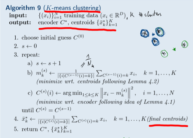
The algorithm (using iterative greedy descent):

Dimensionality Reduction

Since modern ML algorithms can handle very high-dimensional examples, dimensionality reduction techniques are used less in practice than in the past.
The most frequent use case is data visualization: human can only interpret on a plot the maximum of three dimensions.
Another situation is that we need to build an interpretable model and are limited in the choice of algorithms. Then it removes redundant or highly correlated features and also reduces the noise in the data, which all improve the interpretability of the model.

Principal Component Analysis (PCA)

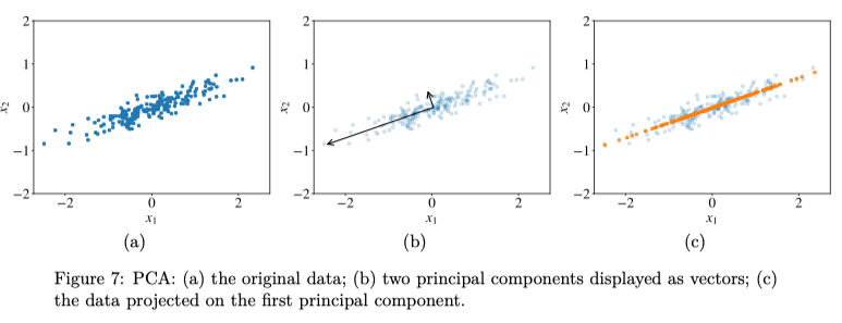
Example:
Principal components are vectors that define a new coordinate system in which the first axis goes in the direction of the highest variance in the data. The second axis is orthogonal to the first one and goes in the direction of the second highest variance in the data. The length of the arrow reflects the variance in the direction. They form the orthogonal basis.
If we want to reduce the dimensionality to $D_{new} < D$, we pick $D_{new}$ largest principal components and project our data points on them. For 2D, we can set $D_{new} = 1$ and get the projected orange points in the figure. To describe each orange point, we need only one coordinate instead of two: the coordinate with respect to the first principal component.
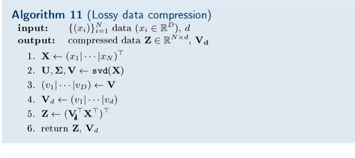
For data compression/ dimensionality reduction, we aim to look for a lower-dimensional representation / compression of data (lossy compression, ${W}_d \ {V}_d$ are matrices for compression and decompression respectively):

$$z_i = comp_d (x_i)$$ $$x_i \approx \hat x_i = decomp_d (z_i)$$ $$(\hat{V_d}, \hat{W_d}) = argmin_{W_d, {V}d} \sum{i=1}^N||x_i-V_d {W}_d x_i||^2$$
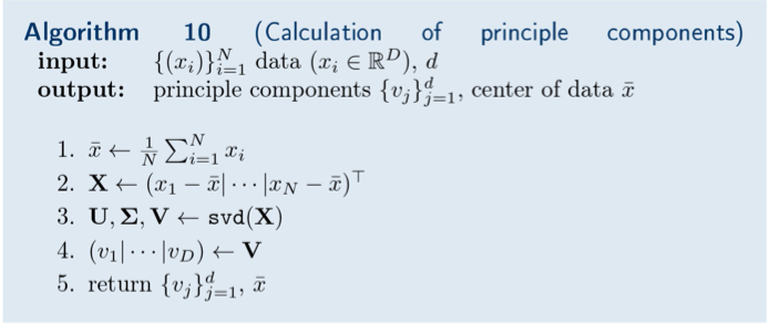
For the matrix above ($\hat{V_d}$), it’s orthonormal and $\hat{W_d} = \hat{V_d^T}$. So we can rewrite our minimization problem (the columns of $\hat {V}_d$ are called principle components, which are ordered by importance):

$$\hat {V_d} = argmin_{V_d} \sum_{i=1}^N||x_i-V_d V_d^T x_i||^2$$
Algorithms (svd -> singular value)